View Jupyter notebook on the GitHub.
Mechanics of forecasting#
![]()
This notebook uncovers the details of forecasting by pipelines in ETNA library. We are going to explain how pipelines are dealing with dataset, transforms and models to make a prediction.
Table of contents
Loading dataset
Forecasting
Context-free models
Context-required models
ML models
Summary
[1]:
!pip install "etna[prophet]" -q
[2]:
import warnings

warnings.filterwarnings("ignore")
[3]:
import pandas as pd

from etna.datasets import TSDataset
1. Loading dataset#
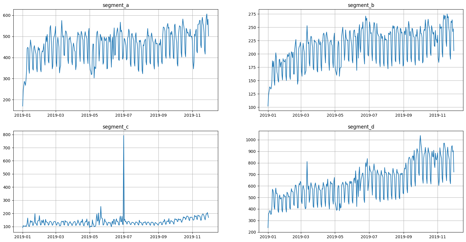
Let’s load and look at the dataset
[4]:
df = pd.read_csv("data/example_dataset.csv")
df.head()
[4]:
| timestamp | segment | target | |
|---|---|---|---|
| 0 | 2019-01-01 | segment_a | 170 |
| 1 | 2019-01-02 | segment_a | 243 |
| 2 | 2019-01-03 | segment_a | 267 |
| 3 | 2019-01-04 | segment_a | 287 |
| 4 | 2019-01-05 | segment_a | 279 |
[5]:
ts = TSDataset(df, freq="D")
ts.plot()
2. Forecasting#
Now let’s dive deeper into forecasting without pipelines. We are going to use only TSDataset, transforms and models.
[6]:
HORIZON = 14
[7]:
train_ts, test_ts = ts.train_test_split(test_size=HORIZON)
[8]:
test_ts.info()
<class 'etna.datasets.TSDataset'>
num_segments: 4
num_exogs: 0
num_regressors: 0
num_known_future: 0
freq: D
end_timestamp: 2019-11-30 00:00:00
          start_timestamp  length  num_missing
segments
segment_a      2019-11-17      14            0
segment_b      2019-11-17      14            0
segment_c      2019-11-17      14            0
segment_d      2019-11-17      14            0
3.1 Context-free models#
Let’s start by using the ProphetModel, because it doesn’t require any transformations and doesn’t need any context.
Fitting the model is very easy
[9]:
from etna.models import ProphetModel

model = ProphetModel()
model.fit(train_ts)
14:49:37 - cmdstanpy - INFO - Chain [1] start processing
14:49:37 - cmdstanpy - INFO - Chain [1] done processing
14:49:38 - cmdstanpy - INFO - Chain [1] start processing
14:49:38 - cmdstanpy - INFO - Chain [1] done processing
14:49:38 - cmdstanpy - INFO - Chain [1] start processing
14:49:38 - cmdstanpy - INFO - Chain [1] done processing
14:49:38 - cmdstanpy - INFO - Chain [1] start processing
14:49:38 - cmdstanpy - INFO - Chain [1] done processing
[9]:
ProphetModel(growth = 'linear', changepoints = None, n_changepoints = 25, changepoint_range = 0.8, yearly_seasonality = 'auto', weekly_seasonality = 'auto', daily_seasonality = 'auto', holidays = None, seasonality_mode = 'additive', seasonality_prior_scale = 10.0, holidays_prior_scale = 10.0, changepoint_prior_scale = 0.05, mcmc_samples = 0, interval_width = 0.8, uncertainty_samples = 1000, stan_backend = None, additional_seasonality_params = (), timestamp_column = None, )
To make a forecast we should create a dataset with future data by using make_future method. We are currently interested in only future_steps parameter, it determines how many timestamps should be created after the end of the history.
As a result we would have a dataset with future_steps timestamps.
[10]:
future_ts = train_ts.make_future(future_steps=HORIZON)
future_ts
[10]:
| segment | segment_a | segment_b | segment_c | segment_d |
|---|---|---|---|---|
| feature | target | target | target | target |
| timestamp | ||||
| 2019-11-17 | NaN | NaN | NaN | NaN |
| 2019-11-18 | NaN | NaN | NaN | NaN |
| 2019-11-19 | NaN | NaN | NaN | NaN |
| 2019-11-20 | NaN | NaN | NaN | NaN |
| 2019-11-21 | NaN | NaN | NaN | NaN |
| 2019-11-22 | NaN | NaN | NaN | NaN |
| 2019-11-23 | NaN | NaN | NaN | NaN |
| 2019-11-24 | NaN | NaN | NaN | NaN |
| 2019-11-25 | NaN | NaN | NaN | NaN |
| 2019-11-26 | NaN | NaN | NaN | NaN |
| 2019-11-27 | NaN | NaN | NaN | NaN |
| 2019-11-28 | NaN | NaN | NaN | NaN |
| 2019-11-29 | NaN | NaN | NaN | NaN |
| 2019-11-30 | NaN | NaN | NaN | NaN |
Now we are ready to make a forecast
[11]:
forecast_ts = model.forecast(future_ts)
forecast_ts
[11]:
| segment | segment_a | segment_b | segment_c | segment_d |
|---|---|---|---|---|
| feature | target | target | target | target |
| timestamp | ||||
| 2019-11-17 | 417.673477 | 196.558737 | 143.788667 | 723.130705 |
| 2019-11-18 | 530.657704 | 248.126734 | 181.274089 | 900.628287 |
| 2019-11-19 | 547.467047 | 252.990611 | 173.441251 | 938.119256 |
| 2019-11-20 | 538.082365 | 248.468823 | 169.359185 | 921.984471 |
| 2019-11-21 | 531.357617 | 244.777693 | 169.557257 | 916.241514 |
| 2019-11-22 | 519.183714 | 240.262203 | 167.973756 | 906.370764 |
| 2019-11-23 | 431.966427 | 203.855615 | 147.703800 | 759.319762 |
| 2019-11-24 | 420.674705 | 197.069259 | 146.028192 | 735.773681 |
| 2019-11-25 | 533.658932 | 248.637256 | 183.513615 | 913.271263 |
| 2019-11-26 | 550.468274 | 253.501133 | 175.680777 | 950.762232 |
| 2019-11-27 | 541.083592 | 248.979345 | 171.598710 | 934.627447 |
| 2019-11-28 | 534.358844 | 245.288215 | 171.796782 | 928.884490 |
| 2019-11-29 | 522.184942 | 240.772725 | 170.213282 | 919.013740 |
| 2019-11-30 | 434.967654 | 204.366137 | 149.943325 | 771.962738 |
We should note that forecast_ts isn’t a new dataset, it is the same object as future_ts, but filled with predicted values
[12]:
forecast_ts is future_ts
[12]:
True
Now let’s look at a metric and plot the prediction.
[13]:
from etna.metrics import SMAPE

smape = SMAPE()
smape(y_true=test_ts, y_pred=forecast_ts)
[13]:
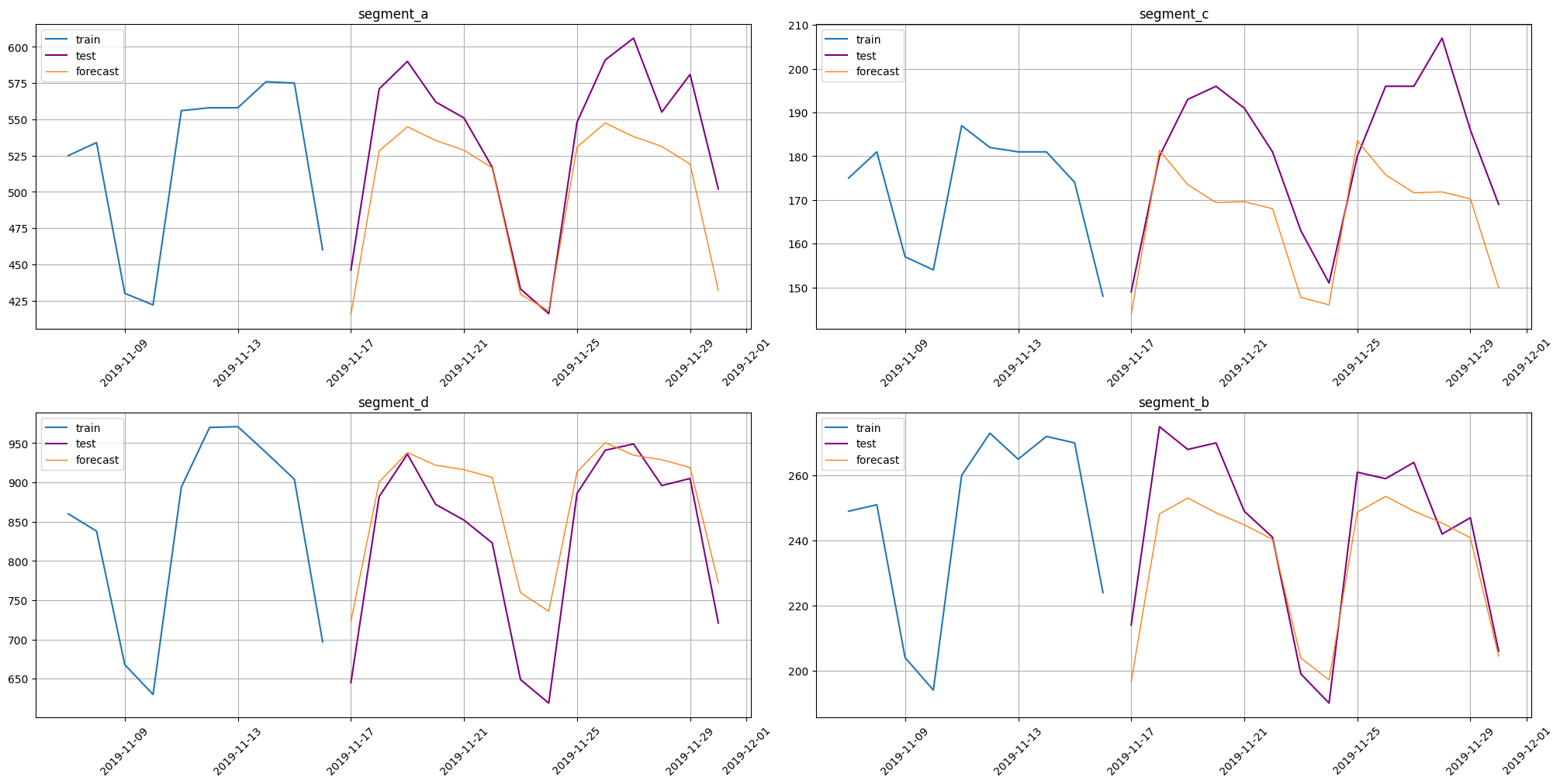
{'segment_a': 5.782173639024761,
 'segment_b': 4.176505858890025,
 'segment_c': 9.115732497272823,
 'segment_d': 6.191490704821549}
[14]:
from etna.analysis import plot_forecast

plot_forecast(forecast_ts, test_ts, train_ts, n_train_samples=10)
3.2 Context-required models#
First of all, let’s clarify that context is. The context is a history data the precedes the forecasting horizon.
And now let’s expand our scheme to models that require some history context for forecasting. The example is NaiveModel, because it needs to know the value lag steps ago.
The fitting doesn’t change
[15]:
from etna.models import NaiveModel

model = NaiveModel(lag=14)
model.fit(train_ts)
[15]:
NaiveModel(lag = 14, )
The models has context_size attribute that in this particular case is equal to lag
[16]:
model.context_size
[16]:
14
Future generation now needs a new parameter: tail_steps, it determines how many timestamps should be created before the end of the history.
The result will contain future_steps + tail_step timestamps.
[17]:
future_ts = train_ts.make_future(future_steps=HORIZON, tail_steps=model.context_size)
future_ts
[17]:
| segment | segment_a | segment_b | segment_c | segment_d |
|---|---|---|---|---|
| feature | target | target | target | target |
| timestamp | ||||
| 2019-11-03 | 346.0 | 184.0 | 149.0 | 604.0 |
| 2019-11-04 | 378.0 | 196.0 | 153.0 | 652.0 |
| 2019-11-05 | 510.0 | 256.0 | 185.0 | 931.0 |
| 2019-11-06 | 501.0 | 248.0 | 178.0 | 885.0 |
| 2019-11-07 | 525.0 | 249.0 | 175.0 | 860.0 |
| 2019-11-08 | 534.0 | 251.0 | 181.0 | 838.0 |
| 2019-11-09 | 430.0 | 204.0 | 157.0 | 668.0 |
| 2019-11-10 | 422.0 | 194.0 | 154.0 | 630.0 |
| 2019-11-11 | 556.0 | 260.0 | 187.0 | 894.0 |
| 2019-11-12 | 558.0 | 273.0 | 182.0 | 970.0 |
| 2019-11-13 | 558.0 | 265.0 | 181.0 | 971.0 |
| 2019-11-14 | 576.0 | 272.0 | 181.0 | 938.0 |
| 2019-11-15 | 575.0 | 270.0 | 174.0 | 904.0 |
| 2019-11-16 | 460.0 | 224.0 | 148.0 | 697.0 |
| 2019-11-17 | NaN | NaN | NaN | NaN |
| 2019-11-18 | NaN | NaN | NaN | NaN |
| 2019-11-19 | NaN | NaN | NaN | NaN |
| 2019-11-20 | NaN | NaN | NaN | NaN |
| 2019-11-21 | NaN | NaN | NaN | NaN |
| 2019-11-22 | NaN | NaN | NaN | NaN |
| 2019-11-23 | NaN | NaN | NaN | NaN |
| 2019-11-24 | NaN | NaN | NaN | NaN |
| 2019-11-25 | NaN | NaN | NaN | NaN |
| 2019-11-26 | NaN | NaN | NaN | NaN |
| 2019-11-27 | NaN | NaN | NaN | NaN |
| 2019-11-28 | NaN | NaN | NaN | NaN |
| 2019-11-29 | NaN | NaN | NaN | NaN |
| 2019-11-30 | NaN | NaN | NaN | NaN |
Forecasting is slightly changed too. We need to pass prediction_size parameter that determines how many timestamps we want to see in our result.
[18]:
forecast_ts = model.forecast(future_ts, prediction_size=HORIZON)
forecast_ts
[18]:
| segment | segment_a | segment_b | segment_c | segment_d |
|---|---|---|---|---|
| feature | target | target | target | target |
| timestamp | ||||
| 2019-11-17 | 346.0 | 184.0 | 149.0 | 604.0 |
| 2019-11-18 | 378.0 | 196.0 | 153.0 | 652.0 |
| 2019-11-19 | 510.0 | 256.0 | 185.0 | 931.0 |
| 2019-11-20 | 501.0 | 248.0 | 178.0 | 885.0 |
| 2019-11-21 | 525.0 | 249.0 | 175.0 | 860.0 |
| 2019-11-22 | 534.0 | 251.0 | 181.0 | 838.0 |
| 2019-11-23 | 430.0 | 204.0 | 157.0 | 668.0 |
| 2019-11-24 | 422.0 | 194.0 | 154.0 | 630.0 |
| 2019-11-25 | 556.0 | 260.0 | 187.0 | 894.0 |
| 2019-11-26 | 558.0 | 273.0 | 182.0 | 970.0 |
| 2019-11-27 | 558.0 | 265.0 | 181.0 | 971.0 |
| 2019-11-28 | 576.0 | 272.0 | 181.0 | 938.0 |
| 2019-11-29 | 575.0 | 270.0 | 174.0 | 904.0 |
| 2019-11-30 | 460.0 | 224.0 | 148.0 | 697.0 |
The forecast_ts and future_ts are still the same object
[19]:
forecast_ts is future_ts
[19]:
True
The result of forecasting
[20]:
smape(y_true=test_ts, y_pred=forecast_ts)
[20]:
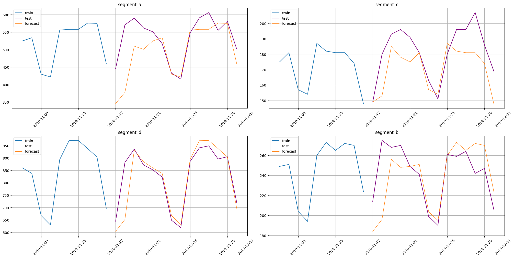
{'segment_a': 9.362036158596007,
 'segment_b': 7.520927594702097,
 'segment_c': 6.930906591160424,
 'segment_d': 4.304033333591803}
[21]:
plot_forecast(forecast_ts, test_ts, train_ts, n_train_samples=10)
3.3 ML models#
Now we are going to expand our scheme even further by using transformations.
Let’s define the transformations
[22]:
from etna.transforms import DateFlagsTransform
from etna.transforms import LagTransform
from etna.transforms import LogTransform
from etna.transforms import SegmentEncoderTransform

log = LogTransform(in_column="target")
seg = SegmentEncoderTransform()
lags = LagTransform(in_column="target", lags=list(range(HORIZON, HORIZON + 3)), out_column="lag")
date_flags = DateFlagsTransform(
    day_number_in_week=True,
    day_number_in_month=False,
    week_number_in_month=False,
    is_weekend=False,
    out_column="date_flag",
)
transforms = [log, lags, date_flags, seg]
Fitting the models requires the transformations to be applied to the dataset
[23]:
train_ts
[23]:
| segment | segment_a | segment_b | segment_c | segment_d |
|---|---|---|---|---|
| feature | target | target | target | target |
| timestamp | ||||
| 2019-01-01 | 170 | 102 | 92 | 238 |
| 2019-01-02 | 243 | 123 | 107 | 358 |
| 2019-01-03 | 267 | 130 | 103 | 366 |
| 2019-01-04 | 287 | 138 | 103 | 385 |
| 2019-01-05 | 279 | 137 | 104 | 384 |
| ... | ... | ... | ... | ... |
| 2019-11-12 | 558 | 273 | 182 | 970 |
| 2019-11-13 | 558 | 265 | 181 | 971 |
| 2019-11-14 | 576 | 272 | 181 | 938 |
| 2019-11-15 | 575 | 270 | 174 | 904 |
| 2019-11-16 | 460 | 224 | 148 | 697 |
320 rows × 4 columns
[24]:
train_ts.fit_transform(transforms)
train_ts
[24]:
| segment | segment_a | segment_b | ... | segment_c | segment_d | ||||||||||||||||
|---|---|---|---|---|---|---|---|---|---|---|---|---|---|---|---|---|---|---|---|---|---|
| feature | date_flag_day_number_in_week | lag_14 | lag_15 | lag_16 | segment_code | target | date_flag_day_number_in_week | lag_14 | lag_15 | lag_16 | ... | lag_15 | lag_16 | segment_code | target | date_flag_day_number_in_week | lag_14 | lag_15 | lag_16 | segment_code | target |
| timestamp | |||||||||||||||||||||
| 2019-01-01 | 1 | NaN | NaN | NaN | 0 | 2.232996 | 1 | NaN | NaN | NaN | ... | NaN | NaN | 2 | 1.968483 | 1 | NaN | NaN | NaN | 3 | 2.378398 |
| 2019-01-02 | 2 | NaN | NaN | NaN | 0 | 2.387390 | 2 | NaN | NaN | NaN | ... | NaN | NaN | 2 | 2.033424 | 2 | NaN | NaN | NaN | 3 | 2.555094 |
| 2019-01-03 | 3 | NaN | NaN | NaN | 0 | 2.428135 | 3 | NaN | NaN | NaN | ... | NaN | NaN | 2 | 2.017033 | 3 | NaN | NaN | NaN | 3 | 2.564666 |
| 2019-01-04 | 4 | NaN | NaN | NaN | 0 | 2.459392 | 4 | NaN | NaN | NaN | ... | NaN | NaN | 2 | 2.017033 | 4 | NaN | NaN | NaN | 3 | 2.586587 |
| 2019-01-05 | 5 | NaN | NaN | NaN | 0 | 2.447158 | 5 | NaN | NaN | NaN | ... | NaN | NaN | 2 | 2.021189 | 5 | NaN | NaN | NaN | 3 | 2.585461 |
| ... | ... | ... | ... | ... | ... | ... | ... | ... | ... | ... | ... | ... | ... | ... | ... | ... | ... | ... | ... | ... | ... |
| 2019-11-12 | 1 | 2.701568 | 2.728354 | 2.698970 | 0 | 2.747412 | 1 | 2.357935 | 2.389166 | 2.332438 | ... | 2.235528 | 2.164353 | 2 | 2.262451 | 1 | 2.921686 | 2.946943 | 2.880814 | 3 | 2.987219 |
| 2019-11-13 | 2 | 2.697229 | 2.701568 | 2.728354 | 0 | 2.747412 | 2 | 2.357935 | 2.357935 | 2.389166 | ... | 2.232996 | 2.235528 | 2 | 2.260071 | 2 | 2.916980 | 2.921686 | 2.946943 | 3 | 2.987666 |
| 2019-11-14 | 3 | 2.700704 | 2.697229 | 2.701568 | 0 | 2.761176 | 3 | 2.346353 | 2.357935 | 2.357935 | ... | 2.235528 | 2.232996 | 2 | 2.260071 | 3 | 2.930440 | 2.916980 | 2.921686 | 3 | 2.972666 |
| 2019-11-15 | 4 | 2.682145 | 2.700704 | 2.697229 | 0 | 2.760422 | 4 | 2.372912 | 2.346353 | 2.357935 | ... | 2.235528 | 2.235528 | 2 | 2.243038 | 4 | 2.948902 | 2.930440 | 2.916980 | 3 | 2.956649 |
| 2019-11-16 | 5 | 2.585461 | 2.682145 | 2.700704 | 0 | 2.663701 | 5 | 2.285557 | 2.372912 | 2.346353 | ... | 2.222716 | 2.235528 | 2 | 2.173186 | 5 | 2.833147 | 2.948902 | 2.930440 | 3 | 2.843855 |
320 rows × 24 columns
As you can see, there are several changes made by the transforms:
Added
date_flag_day_number_in_weekcolumn;Added
lag_14, …,lag_19columns;Added
segment_codecolumn;Logarithm applied to
targetcolumn.
Now we are ready to fit our model
[25]:
from etna.models import CatBoostMultiSegmentModel

model = CatBoostMultiSegmentModel()
model.fit(train_ts)
[25]:
CatBoostMultiSegmentModel(iterations = None, depth = None, learning_rate = None, logging_level = 'Silent', l2_leaf_reg = None, thread_count = None, )
In this case preparing future doesn’t require dealing with the context, all the necessary information is in the features. But we have to deal with transformations by passing them into make_future method.
[26]:
future_ts = train_ts.make_future(future_steps=HORIZON, transforms=transforms)
Making a forecast
[27]:
forecast_ts = model.forecast(future_ts)
forecast_ts
[27]:
| segment | segment_a | segment_b | ... | segment_c | segment_d | ||||||||||||||||
|---|---|---|---|---|---|---|---|---|---|---|---|---|---|---|---|---|---|---|---|---|---|
| feature | date_flag_day_number_in_week | lag_14 | lag_15 | lag_16 | segment_code | target | date_flag_day_number_in_week | lag_14 | lag_15 | lag_16 | ... | lag_15 | lag_16 | segment_code | target | date_flag_day_number_in_week | lag_14 | lag_15 | lag_16 | segment_code | target |
| timestamp | |||||||||||||||||||||
| 2019-11-17 | 6 | 2.540329 | 2.585461 | 2.682145 | 0 | 2.556740 | 6 | 2.267172 | 2.285557 | 2.372912 | ... | 2.184691 | 2.222716 | 2 | 2.174014 | 6 | 2.781755 | 2.833147 | 2.948902 | 3 | 2.819766 |
| 2019-11-18 | 0 | 2.578639 | 2.540329 | 2.585461 | 0 | 2.651815 | 0 | 2.294466 | 2.267172 | 2.285557 | ... | 2.176091 | 2.184691 | 2 | 2.230191 | 0 | 2.814913 | 2.781755 | 2.833147 | 3 | 2.826960 |
| 2019-11-19 | 1 | 2.708421 | 2.578639 | 2.540329 | 0 | 2.687395 | 1 | 2.409933 | 2.294466 | 2.267172 | ... | 2.187521 | 2.176091 | 2 | 2.231492 | 1 | 2.969416 | 2.814913 | 2.781755 | 3 | 2.928302 |
| 2019-11-20 | 2 | 2.700704 | 2.708421 | 2.578639 | 0 | 2.695143 | 2 | 2.396199 | 2.409933 | 2.294466 | ... | 2.269513 | 2.187521 | 2 | 2.233829 | 2 | 2.947434 | 2.969416 | 2.814913 | 3 | 2.942484 |
| 2019-11-21 | 3 | 2.720986 | 2.700704 | 2.708421 | 0 | 2.681276 | 3 | 2.397940 | 2.396199 | 2.409933 | ... | 2.252853 | 2.269513 | 2 | 2.243859 | 3 | 2.935003 | 2.947434 | 2.969416 | 3 | 2.949650 |
| 2019-11-22 | 4 | 2.728354 | 2.720986 | 2.700704 | 0 | 2.687179 | 4 | 2.401401 | 2.397940 | 2.396199 | ... | 2.245513 | 2.252853 | 2 | 2.259357 | 4 | 2.923762 | 2.935003 | 2.947434 | 3 | 2.952880 |
| 2019-11-23 | 5 | 2.634477 | 2.728354 | 2.720986 | 0 | 2.612151 | 5 | 2.311754 | 2.401401 | 2.397940 | ... | 2.260071 | 2.245513 | 2 | 2.191276 | 5 | 2.825426 | 2.923762 | 2.935003 | 3 | 2.840746 |
| 2019-11-24 | 6 | 2.626340 | 2.634477 | 2.728354 | 0 | 2.602040 | 6 | 2.290035 | 2.311754 | 2.401401 | ... | 2.198657 | 2.260071 | 2 | 2.174478 | 6 | 2.800029 | 2.825426 | 2.923762 | 3 | 2.808645 |
| 2019-11-25 | 0 | 2.745855 | 2.626340 | 2.634477 | 0 | 2.704428 | 0 | 2.416641 | 2.290035 | 2.311754 | ... | 2.190332 | 2.198657 | 2 | 2.236019 | 0 | 2.951823 | 2.800029 | 2.825426 | 3 | 2.926138 |
| 2019-11-26 | 1 | 2.747412 | 2.745855 | 2.626340 | 0 | 2.717247 | 1 | 2.437751 | 2.416641 | 2.290035 | ... | 2.274158 | 2.190332 | 2 | 2.250306 | 1 | 2.987219 | 2.951823 | 2.800029 | 3 | 2.941435 |
| 2019-11-27 | 2 | 2.747412 | 2.747412 | 2.745855 | 0 | 2.728090 | 2 | 2.424882 | 2.437751 | 2.416641 | ... | 2.262451 | 2.274158 | 2 | 2.269917 | 2 | 2.987666 | 2.987219 | 2.951823 | 3 | 2.954827 |
| 2019-11-28 | 3 | 2.761176 | 2.747412 | 2.747412 | 0 | 2.741196 | 3 | 2.436163 | 2.424882 | 2.437751 | ... | 2.260071 | 2.262451 | 2 | 2.263858 | 3 | 2.972666 | 2.987666 | 2.987219 | 3 | 2.949533 |
| 2019-11-29 | 4 | 2.760422 | 2.761176 | 2.747412 | 0 | 2.738022 | 4 | 2.432969 | 2.436163 | 2.424882 | ... | 2.260071 | 2.260071 | 2 | 2.239212 | 4 | 2.956649 | 2.972666 | 2.987666 | 3 | 2.949205 |
| 2019-11-30 | 5 | 2.663701 | 2.760422 | 2.761176 | 0 | 2.667598 | 5 | 2.352183 | 2.432969 | 2.436163 | ... | 2.243038 | 2.260071 | 2 | 2.162335 | 5 | 2.843855 | 2.956649 | 2.972666 | 3 | 2.869409 |
14 rows × 24 columns
The forecasted values are too small because we forecasted the target after the logarithm transformation. To get the predictions in original domain we should apply inverse transformation to the predicted values.
[28]:
forecast_ts.inverse_transform(transforms)
forecast_ts
[28]:
| segment | segment_a | segment_b | ... | segment_c | segment_d | ||||||||||||||||
|---|---|---|---|---|---|---|---|---|---|---|---|---|---|---|---|---|---|---|---|---|---|
| feature | date_flag_day_number_in_week | lag_14 | lag_15 | lag_16 | segment_code | target | date_flag_day_number_in_week | lag_14 | lag_15 | lag_16 | ... | lag_15 | lag_16 | segment_code | target | date_flag_day_number_in_week | lag_14 | lag_15 | lag_16 | segment_code | target |
| timestamp | |||||||||||||||||||||
| 2019-11-17 | 6 | 2.540329 | 2.585461 | 2.682145 | 0 | 359.363234 | 6 | 2.267172 | 2.285557 | 2.372912 | ... | 2.184691 | 2.222716 | 2 | 148.284301 | 6 | 2.781755 | 2.833147 | 2.948902 | 3 | 659.338222 |
| 2019-11-18 | 0 | 2.578639 | 2.540329 | 2.585461 | 0 | 447.554679 | 0 | 2.294466 | 2.267172 | 2.285557 | ... | 2.176091 | 2.184691 | 2 | 168.899245 | 0 | 2.814913 | 2.781755 | 2.833147 | 3 | 670.367743 |
| 2019-11-19 | 1 | 2.708421 | 2.578639 | 2.540329 | 0 | 485.849895 | 1 | 2.409933 | 2.294466 | 2.267172 | ... | 2.187521 | 2.176091 | 2 | 169.408727 | 1 | 2.969416 | 2.814913 | 2.781755 | 3 | 846.817556 |
| 2019-11-20 | 2 | 2.700704 | 2.708421 | 2.578639 | 0 | 494.613183 | 2 | 2.396199 | 2.409933 | 2.294466 | ... | 2.269513 | 2.187521 | 2 | 170.328273 | 2 | 2.947434 | 2.969416 | 2.814913 | 3 | 874.959979 |
| 2019-11-21 | 3 | 2.720986 | 2.700704 | 2.708421 | 0 | 479.038925 | 3 | 2.397940 | 2.396199 | 2.409933 | ... | 2.252853 | 2.269513 | 2 | 174.330918 | 3 | 2.935003 | 2.947434 | 2.969416 | 3 | 889.533321 |
| 2019-11-22 | 4 | 2.728354 | 2.720986 | 2.700704 | 0 | 485.607701 | 4 | 2.401401 | 2.397940 | 2.396199 | ... | 2.245513 | 2.252853 | 2 | 180.700706 | 4 | 2.923762 | 2.935003 | 2.947434 | 3 | 896.179874 |
| 2019-11-23 | 5 | 2.634477 | 2.728354 | 2.720986 | 0 | 408.403156 | 5 | 2.311754 | 2.401401 | 2.397940 | ... | 2.260071 | 2.245513 | 2 | 154.337508 | 5 | 2.825426 | 2.923762 | 2.935003 | 3 | 692.020491 |
| 2019-11-24 | 6 | 2.626340 | 2.634477 | 2.728354 | 0 | 398.981966 | 6 | 2.290035 | 2.311754 | 2.401401 | ... | 2.198657 | 2.260071 | 2 | 148.443830 | 6 | 2.800029 | 2.825426 | 2.923762 | 3 | 642.643396 |
| 2019-11-25 | 0 | 2.745855 | 2.626340 | 2.634477 | 0 | 505.323214 | 0 | 2.416641 | 2.290035 | 2.311754 | ... | 2.190332 | 2.198657 | 2 | 171.194270 | 0 | 2.951823 | 2.800029 | 2.825426 | 3 | 842.603449 |
| 2019-11-26 | 1 | 2.747412 | 2.745855 | 2.626340 | 0 | 520.491759 | 1 | 2.437751 | 2.416641 | 2.290035 | ... | 2.274158 | 2.190332 | 2 | 176.953209 | 1 | 2.987219 | 2.951823 | 2.800029 | 3 | 872.846999 |
| 2019-11-27 | 2 | 2.747412 | 2.747412 | 2.745855 | 0 | 533.675426 | 2 | 2.424882 | 2.437751 | 2.416641 | ... | 2.262451 | 2.274158 | 2 | 185.173306 | 2 | 2.987666 | 2.987219 | 2.951823 | 3 | 900.211426 |
| 2019-11-28 | 3 | 2.761176 | 2.747412 | 2.747412 | 0 | 550.055772 | 3 | 2.436163 | 2.424882 | 2.437751 | ... | 2.260071 | 2.262451 | 2 | 182.593736 | 3 | 2.972666 | 2.987666 | 2.987219 | 3 | 889.293412 |
| 2019-11-29 | 4 | 2.760422 | 2.761176 | 2.747412 | 0 | 546.043578 | 4 | 2.432969 | 2.436163 | 2.424882 | ... | 2.260071 | 2.260071 | 2 | 172.465049 | 4 | 2.956649 | 2.972666 | 2.987666 | 3 | 888.621079 |
| 2019-11-30 | 5 | 2.663701 | 2.760422 | 2.761176 | 0 | 464.155824 | 5 | 2.352183 | 2.432969 | 2.436163 | ... | 2.243038 | 2.260071 | 2 | 144.323108 | 5 | 2.843855 | 2.956649 | 2.972666 | 3 | 739.302815 |
14 rows × 24 columns
The result of forecasting
[29]:
smape(y_true=test_ts, y_pred=forecast_ts)
[29]:
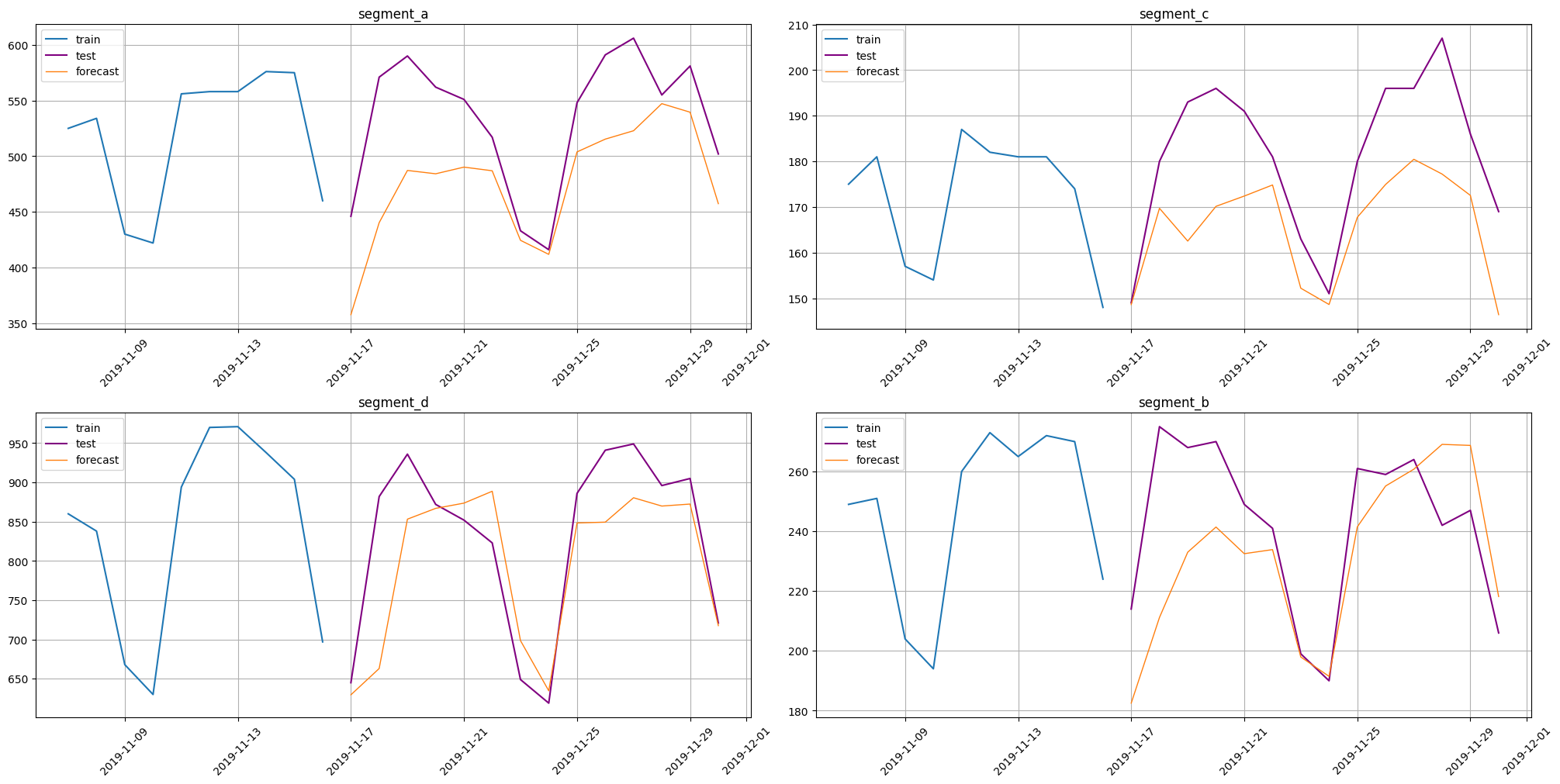
{'segment_a': 11.18164789354642,
 'segment_b': 8.218437980478669,
 'segment_c': 7.648519789798347,
 'segment_d': 6.120890541970104}
[30]:
train_ts.inverse_transform(transforms)
plot_forecast(forecast_ts, test_ts, train_ts, n_train_samples=10)
Summary#
As we can see, pipelines do a lot of work under the hood.
Training:
Applying transformations
Fitting the model
Forecasting:
Generating future dataset with applied transformations
Forecasting with the fitted model
Inverse transformation